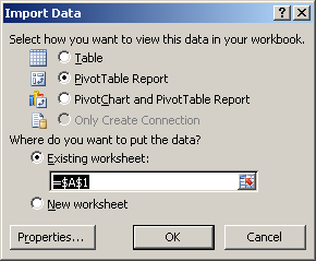
If you chose to import the audit data into an Excel table, in the Import
Data dialog box, select PivotTable Report.
To place the data in the existing worksheet starting at cell A1, leave
Existing worksheet selected:
Click OK.
The resulting, empty PivotTable
appears in the worksheet.
In the PivotTable Field List that appears on the right, select the fields
you want to view.
Tip You can filter data before you add fields. In the PivotTable Field
List, in the Choose fields to add to report box, rest the
pointer on a field name, and then click the filter drop-down arrow next to the field name. On
the Filter menu, select the filter options that you want.
Depending on how you want your PivotTable to be displayed, drag the fields between the areas in the
PivotTable Field List. For example, you may decide to display the names
of the users and the policies that they touched as row labels and actions that the users performed
on policies as column labels.
To be able to filter the PivotTable, under PivotTable Tools,
Options, click Insert Slicer.
In the Insert Slicers dialog box, select the slicers you want to use and
click OK.
You can re-arrange the slicers on the worksheet by selecting a slicer and
dragging and dropping it at a desired position. You can also customize your
slicers, for example, by giving them different colors. To do this, select a
slicer. Under Slicer Tools,
Options, select one of the Slicer
Styles.